


Take a breath. You’re not the only one. Every company running FinOps on Cloudaware has had the same “which numbers really matter?” meeting — usually right after a surprise bill spike and an uncomfortable QBR. Industry data shows teams that formalize KPIs for cloud spend typically see 15–30% cost reductions as they mature their practice.
So this guide cuts through the noise. Below is a short list of battle-tested cloud cost optimization metrics Cloudaware customers use daily, monthly, and quarterly to keep multi-cloud spend predictable, accountable, and defensible.
Steal these 18 metrics, plug them into your tooling, and finally make every review feel like progress, not guesswork.
What cloud cost optimization metrics you track before anything else
Before you dive into unit economics or fancy anomaly models, you need a clean, boringly reliable base layer of cloud cost metrics. This is the stuff your weekly FinOps standups and MBR decks quietly lean on:
- the total monthly cloud spend broken down by provider, account, and project;
- cost by environment so you can see how prod vs non-prod behaves;
- cost by service family across compute, storage, network, and managed databases;
- and your Top N services by spend that explain 60–80% of the bill in one glance.
In the next few sections, we’ll unpack each of these, how to calculate them, and how Cloudaware teams actually use them day-to-day.
Total monthly cloud spend (by provider, account, project)
Before you get fancy with unit economics or anomaly alerts, you came here to answer one brutally simple question: “How much do we spend every month, and where?” Of all the cloud cost metrics you can track, Total monthly cloud spend (by provider, account, project) is the one your CFO, VP Eng, and FinOps lead actually share in slides. And you’re not the only one trying to wrangle it — every company running FinOps on Cloudaware has had this exact “can we just get one true number?” moment.
What the metric is
Total monthly cloud spend is your single, reconciled figure for all public cloud invoices in a given month, broken down by:
- Provider (AWS, Azure, GCP, others).
- Account / subscription / billing profile.
- Project / application / cost center.
The FinOps Foundation even starts its KPI library with high-level spend and allocation indicators, because nothing else works until this one is solid.
How to calculate it
Pick a month. Pick a currency. Then:
- Pull the finalized invoices/billing exports from each provider.
- Decide on a consistent definition of spend. Usually net amortized spend: usage + commitment amortization – provider discounts/credits, excluding taxes and refunds.
- Normalize everything into one currency using your finance-approved FX rates.
- Aggregate totals per provider → per account → per project.
- Reconcile the grand total to your GL / PO-level budget so Finance trusts the number.
In Cloudaware, teams wire this directly from AWS CUR, Azure Cost Management exports, and GCP Billing data, then map accounts to projects via CMDB tags and owner fields, so the hierarchy is always live.
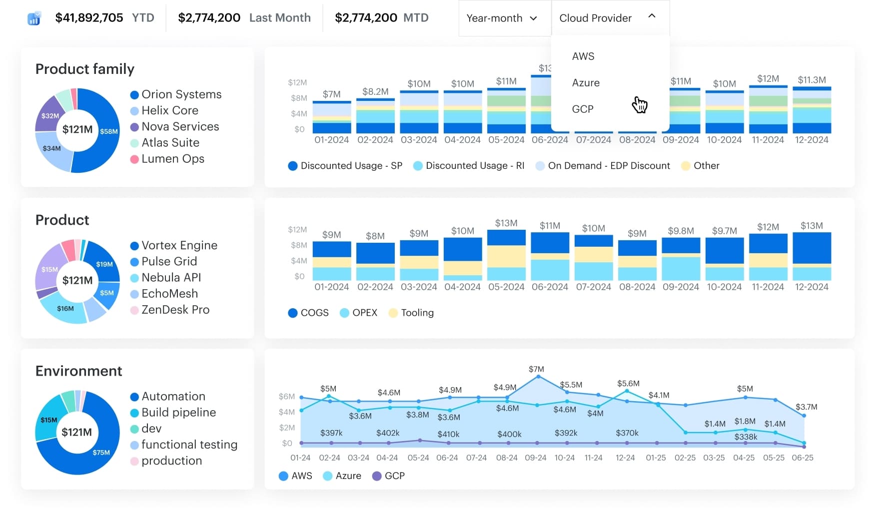
Multi cloud FinOps dashboard in Cloudaware. Schedule a demo to see it live.
What “good” looks like (and how to use it)
Industry studies still show that around 30% of cloud spend goes to waste, thanks to idle resources, overprovisioned instances, and forgotten services. FinOps teams use that as a rough “do better than this” line. Cloudaware customers who are in a healthy spot usually have:
- A reconciled monthly spend number ready within 3–5 business days of month-end.
- MoM variance that leadership can explain (new regions, AI workloads, big launches) instead of “¯\_(ツ)_/¯”.
- Provider/account/project breakdowns that match how budgets and people are organized.
To optimize with this metric, you trend it over time, tie it to budgets, and annotate every spike with a real driver: launch X, new AI cluster, regional expansion, etc. Once that’s in place, you’re ready for the next lens FinOps teams reach for 👇
Cost by environment (prod/non-prod)
Once you’ve nailed the “how much do we spend in total?” question, the next one hits: “Okay, but how much of this is actually serving customers… and how much is just dev, test, and staging humming along at 3 a.m.?”
As cloud cost optimization metrics go, Cost by environment (prod / non-prod) is where ugly truths surface.
Flexera and others keep finding that 25–30% of cloud budgets are pure waste, and a big chunk of that sits in non-production environments left running 24/7. One analysis even showed ~44% of compute spend going to non-prod, which is only needed for a fraction of the workweek.
What the metric is
You’re splitting monthly cloud spend into two big buckets:
- Prod – anything serving real customers or critical internal workloads,
- Non-prod – dev, test, QA, staging, sandboxes, PoCs.
You can keep extra sub-environments if you want, but the core view is binary: what drives revenue vs what supports building and testing it.
How to calculate it
- Standardize your taxonomy. Agree on
environment = prod | non-prodand map any “dev / stage / qa / lab” values into non-prod. - Tag or map every resource. Use tags, account metadata, folders, or projects to assign each line item in AWS CUR, Azure Cost Management, and GCP Billing to an environment.
- Aggregate per month.
- Sum all prod line items → Prod spend
- Sum all non-prod line items → Non-prod spend
- Calculate the share. Non-prod % of total =
Non-prod spend / (Prod + Non-prod)
In Cloudaware, teams usually drive this from a CMDB-backed environment model plus tagging policies, so every instance, database, or function inherits an environment value automatically.
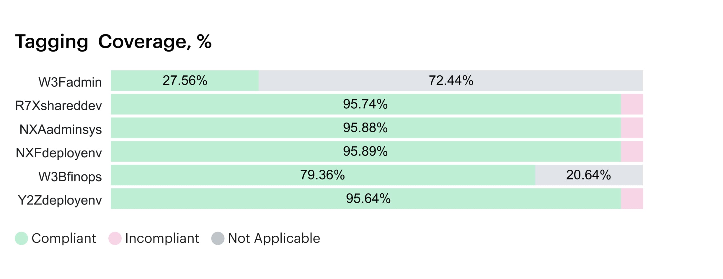
Element of the tagging coverage report in Cloudaware. Schedule a demo to see it live
What “good” looks like
There’s no universal magic ratio, but patterns show up:
- When non-prod creeps above 40–50% of compute spend for long periods, mature FinOps teams treat it as a risk signal, not “just how we work”.
- Healthy orgs can explain their non-prod level in plain language: “We’re running a big migration,” “We have active nightly test runs,” “We spin up heavy perf environments only during release windows.”
- Over time, you want non-prod spend trending flat or down while feature delivery still moves forward. That’s the sign that scheduling, ephemeral environments, and rightsizing are doing their job.
How to use it to optimize spend
This metric is a prioritization engine:
- Spot months where non-prod % jumps and drill into which teams or projects drove it.
- Target scheduling policies at the loudest offenders: shut down dev/test outside business hours, hibernate non-critical clusters over weekends, turn perf environments into “on-demand only”.
- Combine with unit metrics (e.g., non-prod cost per active engineer or per CI pipeline) to show engineering leads exactly what “always-on” really costs.
- Track savings by watching non-prod share fall month over month while delivery velocity stays stable.
Once you can separate where spend happens in the lifecycle (prod vs non-prod), the next move is to see what you’re actually paying for.
Cost by service family (compute, storage, network, managed DB)
Once you’ve split spend by prod and non-prod, the next “oh wow” moment comes when you group it by what you’re actually buying. That’s where Cost by service family (compute, storage, network, managed DB) earns a spot on your shortlist of cloud cost metrics.
You take a month of billing data, map every line item to a family — EC2/VMs/containers/functions into compute, S3/EBS/Blob/GCS into storage, data transfer and load balancers into network, RDS/Cosmos/Cloud SQL into managed DB — then sum each bucket.
Industry analyses show IaaS revenue often skews 60–70% compute, ~20% storage, under 10% networking, with the rest in platform and database services. (Source: Ofcom)
That gives you a rough “is our profile weird?” baseline.
Use this metric to spot noisy categories fast: rising storage without traffic growth, networking jumps from cross-region chatter, or DB spend outpacing active users. From here, zoom into the Top N services by spend to see the culprits by name.
Top N services by spend
You know that moment in the CUR where your eyes glaze over because everything looks expensive? This is where you zoom in with one of the most practical cloud cost optimization metrics you can have: Top N services by spend.
In cloud, a tiny set of providers already captures most of the market, and your bill behaves the same way — a handful of services quietly dominate the total.
Here’s how to work it. Pick a month, aggregate spend by provider + service (EC2, S3, Azure VMs, Cloud SQL, etc.), sort descending, then take the top 10–20 line items. In most environments, that short list explains the bulk of your compute, storage, and database costs.
“Good” looks like:
- No surprises at the top
- Clear owners and use cases for each big service
- Concrete optimization levers per item (commitments, rightsizing, storage tiering, traffic patterns).
This gives you your hit list.
Allocation cloud cost metrics: How much of your cloud bill has an owner?
You can’t run showback on vibes and Slack threads. At some point, someone in Finance will ask, “Who owns this line CI?” and you’ll either have real numbers… or a very long meeting. Allocation is where Cloudaware customers usually move from “we kind of watch the bill” to “we can defend every euro in a room full of VPs.”
Think of these allocation metrics as the backbone of your cloud cost KPIs—the ones that decide whether your dashboards are report-worthy or just screenshots in Confluence.
Allocated spend % (tagged or mapped to app/team/product)
This is the percentage of monthly spend you can confidently tie to a team, app, or product. At month end, you aggregate line items per provider, then sum all entries with valid tags, account mappings, or CMDB scopes and divide by total spend.
FinOps guidance puts mature practices at 80–90% allocation coverage, with Run-level orgs clearing 90%+ consistently.
When you track this across each cloud, it becomes your governance heartbeat: you can see exactly where ownership is slipping, which business units need tagging help, and how ready you are for real showback or chargeback.
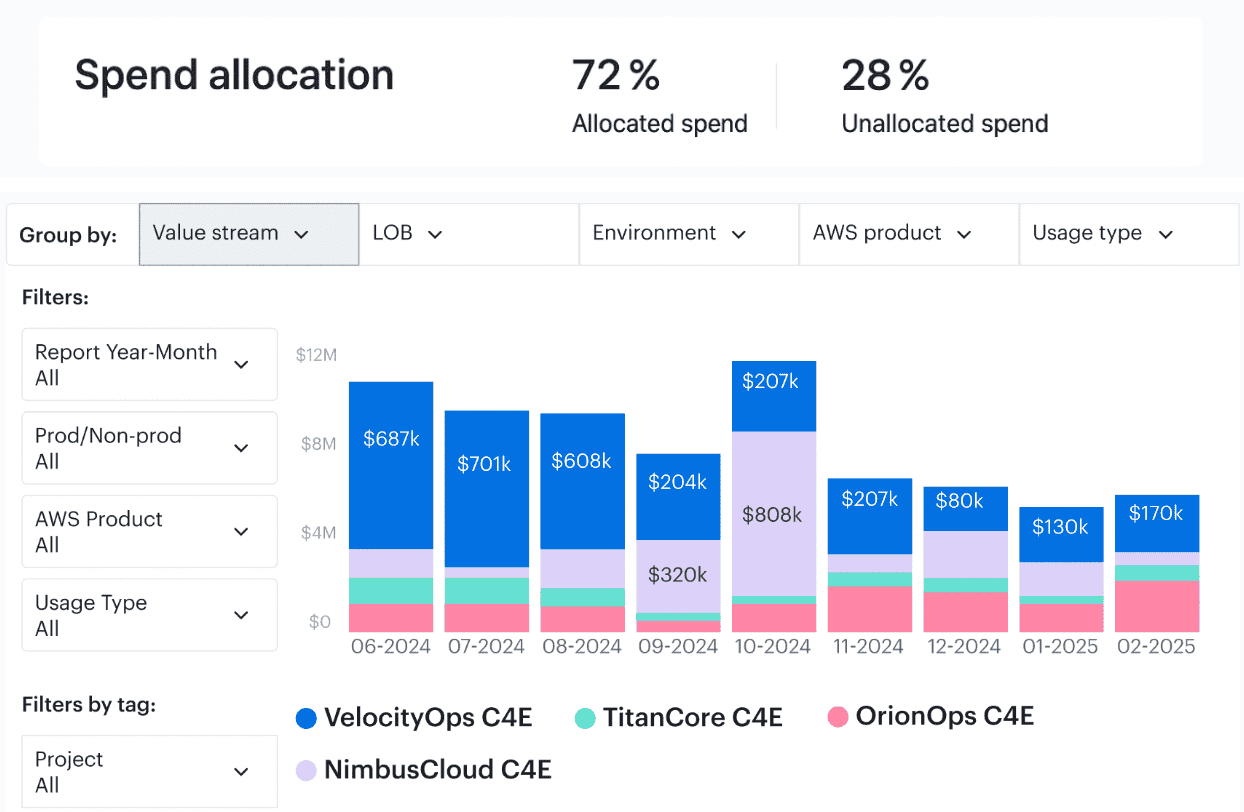
Element of the Cloudaware report of spent allocation history. Schedule a demo to see it live
“Good” looks like: strong growth from 50–60% in the early days toward 80%+ as you standardize tags and hierarchies, then holding above that line even as your footprint expands.
State of FinOps reports show full allocation ranks among the very top priorities for practitioners, right after workload tuning.
That’s your external benchmark for optimization conversations.
Optimally, you wire Allocated % into monthly reviews and QBR decks as the headline allocation cost health metric: if a team wants more infra, you can show exactly how much of their existing estate is already owned, reported, and on the hook.
Unallocated / “mystery” spend %
This is the shadow side of allocation: the percentage of the bill with no owner, no tag, no clear mapping. Calculation is simple – sum all untagged or unmapped line items, divide by total monthly spend, and you’ve got the “mystery” slice that usually hides quick savings.
For many teams, early FinOps maturity means 20–40% of spend is still floating in “other.” As practices mature, published targets push this into low single digits, with some Run-level orgs treating anything above ~5% as an incident to be investigated rather than a normal operating state.
That’s how they keep unmanaged costs from quietly compounding.
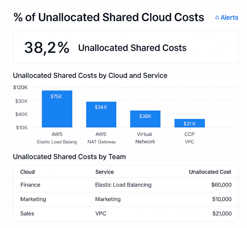
This is an example of a dashboard on unallocated shared costs. Schedule a demo to see it live
The practical play: use Unallocated % as a standing financial risk KPI. Every point you shave off that percentage is real money you can attach to a team, explain in a review, or reduce with a concrete action item instead of arguing over whose budget it should hit.
Shared services allocation coverage (egress, NAT, control planes)
Now for the hard mode: NAT gateways, egress, service meshes, control planes, monitoring, logging, shared Kubernetes clusters, platform teams. Shared services allocation coverage tells you what percentage of those “everyone uses it” items are being distributed back to consumers with an agreed model.
To calculate it, you total shared-service spend, then measure the portion that’s allocated to apps or teams using drivers like requests, traffic, seats, or revenue.
“Good” here means two things: most of your shared spend is allocated, and your model is stable enough that teams trust it. You’ll see this when platform and product leaders start using allocated shared tracking in their own planning instead of keeping shadow spreadsheets.
Shared egress, NAT, or control-plane resources are ingested once, then sliced by owner scopes so showback and chargeback reports feel fair, repeatable, and defensible.
Once these three allocation metrics are in place, your cloud cost reviews stop being “*Where did the money go?_” and start sounding like “_Here’s which teams, services, and shared platforms moved the needle this month.*”
From there, you can finally trust the underlying data, pull out unit economics, and plan serious cost optimization work on top of a bill that’s no longer anonymous.
That’s how you move from reacting to cloud costs to steering them—one allocated percentage point at a time.
Tagging & label data quality metrics
Tag reports are where grown-up FinOps starts. At some point you stop arguing about “*do we even have tags?*” and start asking *“are our tags good enough to show Finance without blushing?*”
That’s the moment tag quality quietly turns into a serious cloud KPI your leadership cares about. FinOps frameworks and tagging guides all repeat the same thing: good tags are the backbone of any allocation, showback, or anomaly story worth sharing.
Mature teams lean on a small set of tag health KPIs as core cloud cost optimization metrics. These sit right beside spend charts on dashboards and QBR decks because they explain how trustworthy every number on the screen really is.
Tagging / label coverage % by spend
What share of your monthly bill is covered by meaningful tags or labels across AWS tags, Azure tags, and GCP labels, across your entire cloud estate? It tells you how much of the invoice can even participate in allocation, showback, and anomaly investigations.
To calculate it, take your billing export, keep only line items where required tag keys from your standard taxonomy exist, sum those amounts, and divide by the overall total. That ratio, multiplied by 100, is your tagging coverage by spend.
Once that number climbs, every optimization discussion with engineering and product has a concrete baseline instead of hand-waving.
In practice, Cloudaware customers get nervous when coverage stays under 60% for long; below that, any story you tell about usage and cost is stitched together from guesses and manual spreadsheets.
State of FinOps surveys and vendor guides commonly cite 80–90% coverage by spend as the bar for reliable allocation and showback.
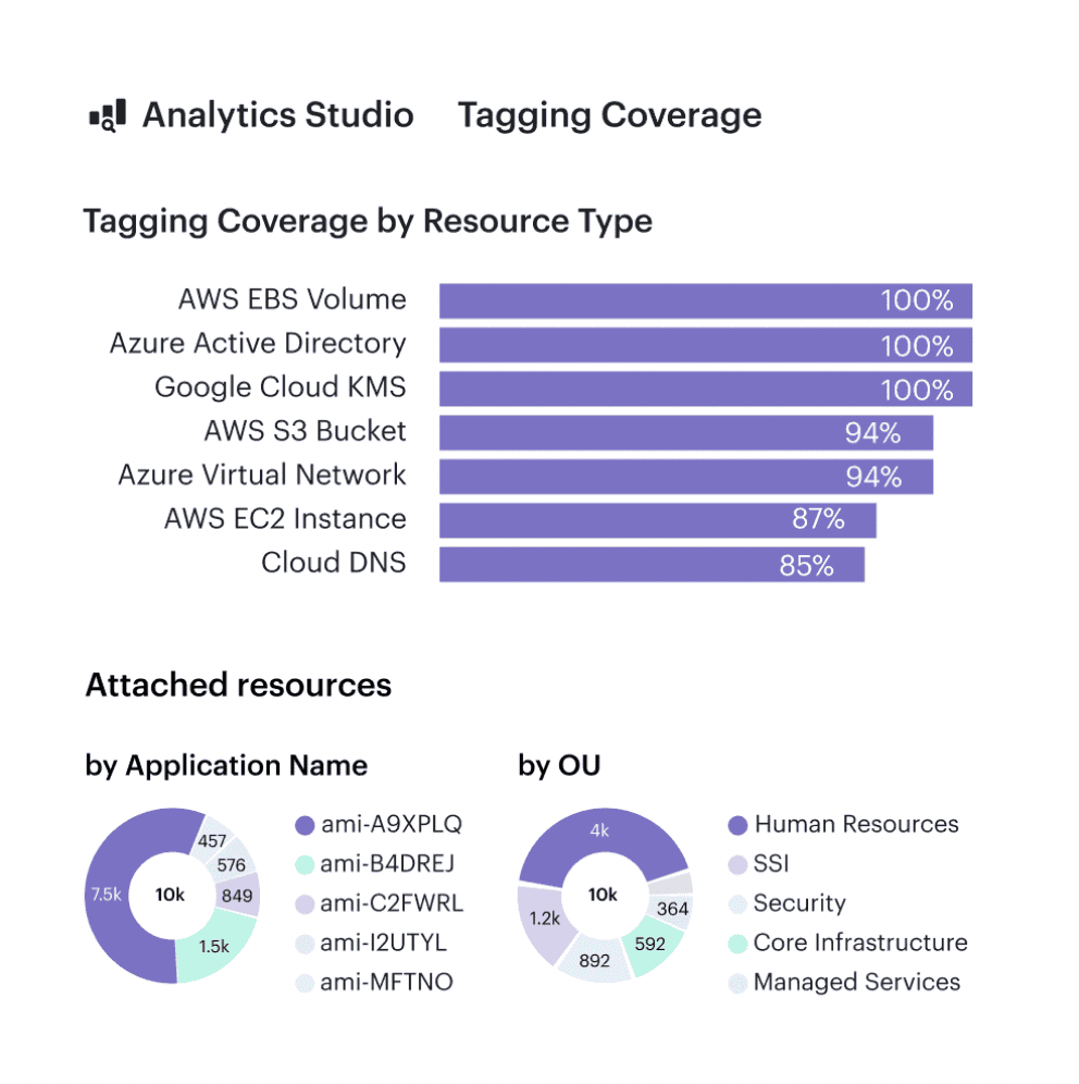
Cloudaware tagging report. Any questions about how it works? Ask us on a live call
Set this metric as a quarterly goal for the platform and FinOps teams: increase coverage by tightening tag standards, backfilling historical records, and enforcing tags during creation through policies and Infrastructure as Code (IaC). Every point you gain usually exposes quick savings, because poorly tagged estates tend to hide idle instances, forgotten volumes, and zombie services.
% of resources with required tags (app, env, owner, cost center)
This view ignores money for a second and looks at hygiene object by object. Out of all running assets in your inventory, what percentage carries the full mandatory tag set—application, environment, owner, and cost center?
Without that baseline, infrastructure sprawl accumulates quiet costs that nobody can point to during reviews.
The math is simple:
- count total items in your inventory snapshot;
- count how many have all required keys present;
- divide and multiply by 100.
That percentage is easy to show to your financial partners because it reads like a compliance score they already understand. Most teams instrument this with AWS Config rules, Azure Policy, and GCP Organization Policies plus scheduled checks.
Teams targeting mature showback generally hold this above the mid-80s in production and push toward the 90s for critical workloads. When it drops, feature teams start losing credibility in budget conversations because no one can prove which application is driving which part of the bill.
Use this metric as an enforcement loop for tag standards: expose it on per-team dashboards, wire checks into CI/CD, and fail pipelines that would lower the overall tagging tracking score for a given service. That’s how tagging stops being a “someone should fix this” task and becomes part of the delivery workflow.
Tag hygiene score (missing/invalid/inconsistent values)
Tag hygiene looks beyond presence to quality:
- Are owners real people or dead lists?
- Are environment values standard?
- Are application names consistent enough that platform teams can line them up with CMDB scopes and shared resources?
A typical approach is to define rules for valid owners, allowed environments, and accepted app names, then scan billing exports plus CMDB inventory. The share of spend with clean, rule-compliant tags becomes your hygiene score and feeds directly into every cloud cost analytics view your FinOps team publishes.
Example of the dashboard with tagging coverage within Cloudaware.
When that score lives in the 90–95% range for production, anomaly detection, showback, and unit-economics models finally get trustworthy data instead of mystery buckets. Tagging stops being a one-off cleanup project and starts acting like a real quality gate.
That’s also where serious cost optimization work starts to pay off. With clean tags, you can slice commitments by product, validate discount coverage per team, and run experiments on environments or architectures without losing the ability to compare before and after.
Waste & rightsizing cloud cost optimization metrics
At some point your FinOps channel hits the same question: “Where exactly is our waste hiding, and how much money is stuck in over-sized stuff?” That’s when the dashboards shift from generic spend views to a sharper bundle of cloud cost optimization metrics, focused purely on waste and rightsizing.
Industry studies consistently show roughly 27–35% of infrastructure spend getting burned on idle or underused capacity—stopped VMs, unattached disks, over-sized instances, and non-prod environments that never sleep.
Once you see those numbers in your own estate, it's hard to un-see them. Especially in a large cloud footprint where hundreds of accounts, subscriptions, and projects all have different habits around size, uptime, and hygiene.
% of spend on idle capacity (stopped VMs, unattached volumes, idle IPs)
This metric measures how much monthly spend goes to stopped compute, unattached storage, idle IPs, and other artifacts that could disappear tomorrow with zero impact.
You calculate it by flagging every line item matching those idle states across providers, summing that amount, and dividing by total monthly spend. That ratio becomes your headline for rightsizing and optimization conversations.
Native advisors in the major platforms focus heavily on this category because it is the safest, least controversial place to start trimming waste.
For benchmarks, mature FinOps teams I talk to try to keep idle spend comfortably in the single digits; when a scan shows 15–20% of the bill tied to idle artifacts, they treat it as a regression.
That’s where the word cost starts to sting in QBR slides, because leaders know this is self-inflicted rather than strategic investment. Flexera’s 2024 report puts average waste around 27% of spend for large estates, which is why this metric shows up in almost every first FinOps clean-up wave.
In practice, you throw this view straight into an “idle clean-up” backlog, sort by team, and attach owners.
Any questions on how it works within Cloudaware? Schedule a free call with our expert
Every ticket has a simple rule of thumb: delete, downsize, or schedule. That backlog often delivers your earliest, least controversial wins, and it gets engineers used to the idea that unused infrastructure is technical debt with a price tag.
Over a few cycles, you should see the idle share trend down even as usage grows; that’s exactly how high-performing teams keep their underlying costs predictable while still shipping features.
Under-utilized instances % (CPU/RAM thresholds)
As soon as the low-hanging idle work is done, leaders start asking about instances that are technically “in use” but still heavily over-provisioned. That’s where under-utilized instance percentage becomes your financial efficiency radar: out of all running VMs, containers, and managed nodes, how many consistently sit well below the capacity you’re paying for?
Most teams follow vendor guidance here—AWS and others often suggest treating anything with max CPU and memory below roughly 40% over a four-week window as a downsizing candidate.
You pull utilization metrics from your monitoring stack, join them with billing exports, mark candidates, then compute the share of spend tied to those instances.
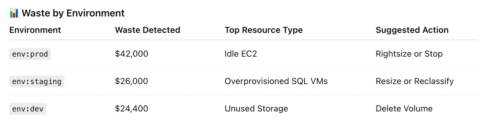
Element of the waste detected report in Cloudaware. Schedule a demo to see it live
That percentage feeds directly into budget discussions around whether you’re designing for performance or just over-buying capacity.
The goal isn’t zero under-utilization. You still want headroom for spikes and deployments. What “good” looks like is a steady reduction in that percentage as you roll through rightsizing waves and autoscaling, plus clear tracking by owner and service, so nobody is surprised when a big node class gets downsized.
Once this metric is visible per product, Cloudaware customers usually sort by spend and start quarterly rightsizing campaigns:
- top offenders first,
- then long-running test systems,
- then shared platform resources like build agents or message brokers that quietly chew through capacity.
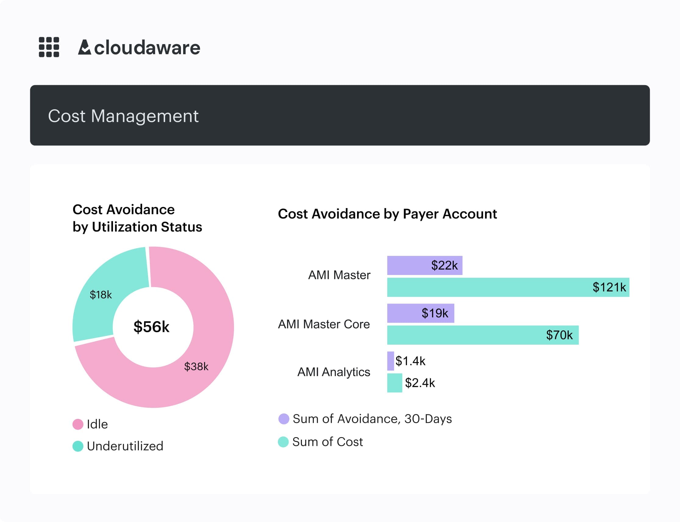
Potential vs realized rightsizing benefit ($)
Here’s where things get real with leadership: the gap between “What a rightsizing engine says you could save” and “what you actually executed”. Potential vs realized rightsizing number takes the theoretical benefit from compute optimizers and compares it to changes that actually hit the bill, giving you a before/after cloud cost story that’s hard to argue with.
You calculate it by aggregating all active rightsizing recommendations into a monthly potential dollar total, then logging implemented changes and measuring the delta in the next few billing cycles.
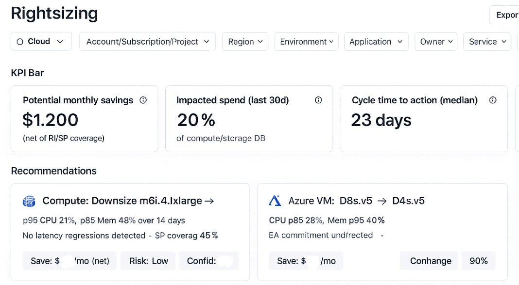
Example of the rightsizing dashboard in Cloudaware. Schedule a demo to see it live
Over time, you’re not just watching recommendations exist—you’re collecting hard data on how fast each team turns advice into lower spend.
Mature teams build this straight into their tuning backlog: every sprint, they pull in a small, prioritized batch of changes and aim for a healthy ratio of realized to potential benefit. When that ratio trends up, it’s a clear sign your cost optimization process is actually moving money, not just generating Jira noise.
Non-prod spend ratio and savings from shutdown schedules
The last lever in this set focuses on environments that don’t need to run 24/7—dev, test, QA, demo. Non-prod spend ratio combined with the impact of scheduled shutdowns answers a simple question: how much of our bill could drop overnight if these systems slept outside office hours?
Case studies and FinOps guidance show that companies automating shutdowns for non-essential environments often cut that slice of cloud costs by 40–65% without any change to delivery speed.
To calculate the ratio, you separate monthly spend into production and non-production buckets, then express the latter as a percentage of the whole. From there, you model weekday-only runtimes or office-hours schedules and track how much spend drops after automation goes live.
Teams in a healthy spot usually see non-prod usage shrink over a few quarters while release cadence stays flat or improves, which tells you scheduling policy is working rather than slowing engineers down.
Taken together, these views give you a clean playbook: run rightsizing waves from the top of your idle and under-utilized lists, keep a standing backlog of the most impactful changes, and let automation handle the nightly and weekend shutdowns.
That’s how FinOps teams using Cloudaware turn one-off clean-ups into a steady habit that keeps the bill lean even as the platform grows.
Commitment & discount metrics (RI, Savings Plans, EA)
You’ve already pulled CUR exports, grouped spend by account and service, argued over dimensions… and you’re still not sure which cloud usage cost metrics actually prove that RIs and Savings Plans are worth the headache.
The FinOps Framework literally calls commitment discounts one of the primary levers in its Rate Optimization capability, so this is where a lot of real money moves.
Every Cloudaware customer I talk to has gone through the same awkward season: weeks of spreadsheet tracking, manually modeling commit levels, and still not having a narrative Finance will sign off on.
You’re not behind; you’re just at the “let’s stop guessing” phase of FinOps maturity.
These four commitment metrics are how the grown-up teams answer, “Are we committing the right amount, in the right places, at the right time?” Let’s break them down one by one.
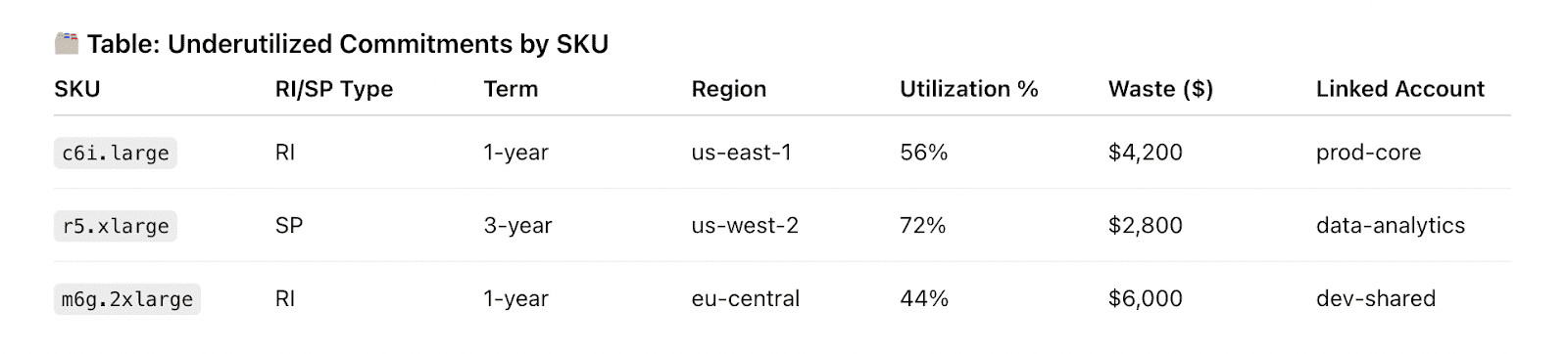
RI / SP coverage % by service/region
RI / SP coverage tells you what portion of eligible compute in your cloud footprint is actually billed at discounted rates for a given service and region. Think: “Of all the EC2 in us-east-1 that could be covered, how much is covered by RIs or Savings Plans?”
To calculate it, take the amortized commitment spend for that service/region and divide it by the on-demand equivalent amount for the same usage period, using your billing data (CUR, AWS Billing Conductor, Azure reservations reports, GCP CUD reports, etc.).
Many practitioners aim for roughly 70–90% coverage on steady-state compute. AWS and independent guides commonly highlight 80–85% coverage as a healthy band for mature environments.
You’ll tune that based on your risk posture and how volatile workloads are.
Once you’re watching coverage by service and region, you can plan your next wave of rate optimization surgically: increase coverage where usage is flat, reduce or avoid new commits where you see churn, and keep this view in front of engineering so they understand where architectural changes impact shared commit pools.
RI / SP utilization %
Utilization measures how much of what you bought is actually being used to generate savings instead of quietly burning in the background. Low utilization is where “cheap rates” turn into very expensive decoration on a dashboard.
Formula: take the value of usage that matched your commitments over the period and divide it by the maximum value those commitments could have covered.
The FinOps Foundation bakes utilization directly into the Effective Savings Rate (ESR) formula alongside coverage and discount rate, which is why under-used commitments tank realized benefit so quickly.
In practice, teams target ~95–100% utilization at the portfolio level, accepting lower utilization in places where big migrations are coming.
A part of the Cloudaware report. Schedule a demo to see it live
When you see utilization sag on a specific service, region, or account, feed it into your costs and commitments review: can you modify, exchange, or resell some portion, or should workloads be shifted back under those discounts?
ESR dashboards make those calls obvious by showing where utilization drag is kneecapping your theoretical discounts.
From there, you fold utilization work into your cost optimization backlog: commitment tuning becomes a recurring practice tied to roadmap changes, not a once-a-year panic before renewals.
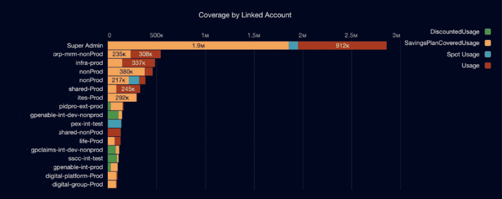
On-demand vs discounted spend ratio
This ratio tells you what share of your overall cloud cost is still running at full on-demand pricing versus commitments, CUDs, or Spot. If a massive chunk of compute keeps landing in the on-demand bucket, you’re leaving a lot of money on the table.
You calculate it by taking all spend billed at on-demand rates for the period and dividing it by total eligible compute spend for the same slice.
Because AWS RIs and Savings Plans can deliver up to ~72% lower prices than on-demand when aligned with usage, leaving a high on-demand share in stable workloads is extremely expensive “optionality.”
This is where your financial partners start paying attention: the ratio is easy to grasp and directly tied to realized ROI on commitments.
This is also the number that rolls nicely into budget season. You can show, “We’re currently at 45% on-demand for compute; if we safely move to 25% while keeping enough headroom for experimentation, here’s the modeled annual impact.”
For multi-year commits, that story continues into renewal cycles and multi-cloud strategy decisions—how much commit headroom do you want per provider, per major program.
Effective hourly rate vs list rate
Finally, effective hourly cost vs list rate is how you sanity-check whether all of this complexity is actually worth it. You take amortized spend for a service (including commitments and any upfront) over a period and divide by actual used hours, then compare that effective rate against the published on-demand price for the same usage.
AWS and ProsperOps frame this in terms of ESR—treating it like ROI on your commitment portfolio.
When you line up effective hourly rates across services and providers, you see which commitments truly reduce cloud costs and which looked attractive on paper but under-delivered because of utilization or coverage gaps.
That view makes “should we renew, expand, or shrink this commit block?” a quantitative discussion instead of gut feel.
Put together, these four metrics give you a clean story for engineering, Finance, and execs: how aggressively you’re committing, how well you’re using what you bought, and how that translates into freed-up resources for new initiatives instead of dead money in the bill.
Once that story is in place, layering on Spot, multi-year deals, and more advanced commitment strategies becomes a controlled experiment—not a gamble.
Budget & forecast accuracy metrics
When you walk into a planning call with your CFO, you’re suddenly judged on a different scoreboard—cloud cost KPIs, not just uptime graphs, ticket queues, or deployment velocity.
Those conversations only get harder as your estate grows; in a modern cloud, a single feature launch can move millions per year if nobody connects roadmap decisions to what will show up in next quarter’s invoice.
Budget vs actual variance % (per team/app/provider)
Budget vs actual variance is the metric that answers, “Did this team, app, or provider land roughly where they promised?” This metric becomes the line item that every engineering leader must defend when next year’s budget is discussed.
To calculate it, you take the planned spend per team, application, and provider for the month, subtract what actually hit the bill, divide by the plan, and express the result as a percentage. Run that consistently across AWS, Azure, and GCP billing exports so it is always backed by the same data your controllers see in the ledger.
The FinOps Framework’s forecasting guidance talks about acceptable variance bands—around 20% for early programs, trending toward 12–15% as practices mature. It roughly matches what most financial partners consider “good enough to run the company on” for a highly variable utility like public infrastructure.
When this metric keeps drifting high and in one direction, you have a ready-made agenda: dig into the workloads, architecture changes, and pricing events behind each spike and turn those explanations into concrete actions before that pattern hardens into permanent cost in the run rate.
Forecast accuracy % (M+1 / Q+1)
Forecast accuracy picks up the story from there. It tells you how sharp your aim is when you look one month or one quarter ahead, and becomes the simplest tracking number you can put in front of executives who just want to know, “How often do you get this right?”
Practically, you take the absolute percentage difference between forecast and actual for the period, subtract that from 100, and the result is your accuracy score.

If you forecast 50,000 and end up at 52,000, you’re sitting at 96% accuracy, which makes any future cloud cost scenario you bring into a steering meeting feel far less like a guess and far more like a controlled experiment.
State of FinOps surveys and case studies show mature programs shrinking variance into single digits, and once your accuracy trend lives there for a few quarters, your QBRs stop revolving around surprise invoices and instead focus on which cost optimization levers—commitments, architecture, or product bets—you want to pull next.
Spend volatility (MoM % change by service or team)
Spend volatility asks a slightly different question: how violently do your monthly costs move by team or major service even when revenue, traffic, and product plans are fairly steady.
To build it, you group spend by service or team, calculate simple month-over-month percentage changes over the last six to twelve periods. Then annotate those lines with events like migrations, launches, or new shared resources coming online so that pattern shifts always connect back to changes in the real world.
FinOps playbooks won’t give you a single magic threshold here, but in practice you want most critical portfolios in a modest volatility band, with big swings reserved for planned projects. That stabilises negotiations with business stakeholders and providers, because any realised savings from tuning architectures or commitments are unlikely to evaporate in the next billing cycle.
When you stitch variance, accuracy, and volatility together, you end up with a forecasting practice that feeds business planning and Finance reporting instead of fighting it.
Every new feature, region, or migration comes with a clearer forward view, and that level of optimization is exactly what gets leadership comfortable saying yes to more experiments instead of cutting back on ambition.
Unit economics & cloud usage cost metrics
You’re in that fun spot where “unit economics” is now a real agenda item, not just a slide. Finance wants levers, Product wants guardrails, Engineering wants something more helpful than “please reduce spend,” and you’re the one in the middle trying to pick the first cloud usage cost metrics that won’t implode under scrutiny.
FinOps best practices all point in the same direction: start by tying infrastructure to business units like customers, transactions, and usage slices.
Let’s walk through four battle-tested unit metrics Cloudaware customers actually use for SaaS margin reviews and pricing decisions:
- Cost per customer / tenant
- Cost per transaction / API call / order
- Cost per GB stored / processed / transferred
- Cost per CI/CD run or data pipeline execution
We’ll unpack how to calculate each one, what “good” looks like in practice, and where to plug them into your SaaS margin analysis, product pricing conversations, and internal SLAs.
Cost per customer / tenant
Think of this as your first deep lens into how your cloud footprint maps to each paying account. Most unit economics guides call cost-per-customer the easiest starting point for connecting infra to revenue streams.
How to calculate: Take total monthly infrastructure spend for a product or tenant-aware stack (all relevant accounts, regions, and shared components you can reasonably allocate), divide it by the active customer count for the same period.
In Cloudaware, that typically means: filter spend by product tag/scope → pull tagged usage into a customer dimension → divide by active tenants flowing in from your CRM or billing export.
Cloudaware FinOps dashboard element. Schedule a demo to see it live
What “good” looks like: You’re looking for trends, not a magic benchmark. Good means:
- You can chart this per cohort (SMB vs enterprise, free vs paid) and see clear differences.
- You can see when a new feature, migration, or architecture change moves the per-customer number up or down in a meaningful way.
Once you can see per-customer economics, you can:
- Flag segments that are expensive to serve and feed that into packaging decisions.
- Pair the metric with ARPU or ARR per customer to watch gross margin drift over time.
This is usually the metric you take into your first serious cloud unit economics review with Product and Finance.
Cost per transaction / API call / order
Next level: zoom in from “per customer” to each billable or value-carrying event. FinOps Foundation explicitly calls out cost-per-transaction as a core unit lens for cloud platforms and APIs.
How to calculate: Pick a clear “unit”: order, API call, search query, streamed minute. Sum infra spend for the services that power that flow (compute, queues, gateways, DB calls) over a period and divide by total transaction volume from your product analytics or event log.
The trick is to use the same time window and definition of “transaction” across teams so the number stands up in reviews about optimization and scaling.
What “good” looks like: You can identify outliers: certain APIs, SKUs, or workloads with a much higher unit rate than the rest. Over a few months, you should see stability or gradual improvement, not wild swings you can’t explain.
Cost per transaction is how you sanity-check new features, promotions, or traffic patterns. Pair it with conversion funnels and latency SLOs to decide where to refactor, where to throttle, and where you’re totally fine spending more to win more volume.
Cost per GB stored / processed / transferred
This family of metrics underpins any data-heavy SaaS: logs, analytics, ML, backups, streaming, you name it. Cloud and FinOps vendors consistently point to per-GB economics as one of the most actionable unit levers for storage-driven platforms.
How to calculate: Decide which layer you’re looking at: stored, processed, or transferred. Then:
- Sum infra spend for the relevant storage, analytics, or network services over the period.
- Divide by total GB for that same dimension (TB written, GB scanned, GB egress, etc.) pulled from native usage metrics or your warehouse.
What “good” looks like
Per-GB numbers that:
- Are broken down by hot / warm / cold tiers so Engineering can see when a dataset should move.
- Make sense against vendor published prices and your own discount structure, so any spike is immediately obvious as architectural, not pricing noise.
This metric is your best friend during cost reviews of analytics features and “let’s store everything forever” habits. It feeds prioritization for compression, retention policies, tiering, and vendor negotiations.
Cost per CI/CD run or data pipeline execution
Finally, the metric that gets Engineering teams to lean in: how much you spend every time a pipeline or deploy runs. Thoughtful unit economics work already calls out cost-per-deployment as a powerful FinOps lever for high-velocity teams.
How to calculate: Pick the system of record for executions (GitHub Actions, GitLab, Jenkins, Airflow, dbt, etc.). For each pipeline category, sum the infra and tooling spend behind those runs—build agents, ephemeral clusters, orchestration services—then divide by total successful executions in the period.
What “good” looks like: You don’t aim for “as low as possible”; you aim for a number that matches the value of having that pipeline. Good looks like:
- Reasonable variance between teams, explained by differences in test depth or workload type.
- A clear link between over-engineered pipelines and elevated per-run spend.
Once you bring cost per run into savings conversations, you can challenge always-on integration, over-parallelized test suites, or redundant staging pipelines without sounding like you’re attacking quality. It becomes a lever in internal SLAs: “For this product, we’re comfortable spending X per deploy for Y reliability and lead time.”
Performance & efficiency metrics (cost vs work done)
Once you’ve got uptime and latency under control, the next set of numbers that quietly decide whether you’re a hero or the person who blew the bill are the money metrics. The ones that turn vague “infra spend” into specific, comparable cloud KPI examples your SRE and DevOps teams can actually act on.
These unit rates tell you, in plain language, how efficiently your workloads are using the underlying cloud and how painful a new feature or traffic spike will be when it hits production.
Cost per 1k requests or RPS
To get this number, pick an endpoint, gateway, or service, take the total spend for it over a period, divide by the number of requests it served, then multiply by 1,000. If your observability stack exposes average requests per second, you can back into the same value by translating RPS into monthly volume first.
Once it’s on a chart right next to latency and error-rate SLIs, it becomes one of your strongest levers for traffic-path optimization because you can instantly see which hops are disproportionately expensive for the value they deliver.
Good for this metric shows up as a shape rather than a single magic number: a relatively flat or gently declining line while your availability and p95 latency stay green.
When you refactor a chatty microservice, introduce caching, or move low-value traffic to a cheaper tier, you want to see the cost per 1k calls drop and stay down across at least a few deploys. If the line bounces back up under peak traffic, that change didn’t really stick and deserves a post-deployment review.
Cost per CPU hour / vCPU
This unit metric tells you how pricey it is to give your workloads CPU time. Combine billing data for a group of instances or a Kubernetes node pool, divide by the total vCPU-hours over the same window, and you have a clean, comparable rate.
SREs love this view because it’s where they uncover the sneaky savings hiding in always-on test environments, oversized workers, or legacy jobs that could easily be pushed to a lower-priority tier.
When you graph this per service or namespace, a healthy pattern is simple: CPU unit costs drift down over time while reliability targets and latency SLOs stay intact. If the rate shoots up with no corresponding improvement in reliability, you probably scaled up just to feel safe.
That’s your cue to experiment with different instance families, adjust autoscaling thresholds, or introduce commitments and then bake the winning configuration into your standard runbooks.
Cost per GB of RAM
The GB-of-RAM metric shines for memory-hungry stacks like JVM services, big in-memory caches, or analytic engines that love to hoard data. Add up everything you’re paying for memory-priced instances in a service, divide by the total GB-hours of RAM provisioned, and you’ll spot workloads treating memory as an infinite buffet rather than a constrained financial asset.
For this one, “good” looks like stable tail latencies and zero swapping alerts while the per-GB rate trends down with each tuning cycle.
When the line spikes, it’s a sign to dig into p95 and p99 memory; maybe a feature toggled on a heavy code path, or a library upgrade introduced a leak.
Use those investigations to set guardrails—heap sizing guidelines, limits in Helm charts, JVM flags—so teams keep their apps fast without blowing up the memory budget every time they ship something big.
Cost per Kubernetes node/pod or per workload
At the platform layer, those same ideas roll up into a view that keeps multi-tenant clusters sane. Take what you’re paying for the underlying worker nodes, control plane, and attached storage, divide by node-hours or pod-hours for a namespace, team, or workload, and you get a unit rate you can use in capacity reviews.
Suddenly platform engineering has a neutral way of tracking which teams are running lean and which ones are endlessly cranking replicas without refactoring anything.
In practice, you turn this into “price per workload” in review decks with SRE, platform, and product: over a few sprints, you ship performance work, the per-workload rate falls, and SLOs remain happy.
That gives you data to enforce minimum and maximum requests, limits to prevent noisy neighbours, and opinionated defaults in your internal templates.
The result is a cluster where teams can ship quickly, incidents stay boring, and you consistently squeeze more value from the same underlying resources.
Anomaly & operational metrics: how fast you react
When your AWS/Azure/GCP bill suddenly jumps and you have no idea why, that’s when all the pretty cloud cost KPIs either save you… or completely abandon you.
This whole block is about the “oh sh*t” moments: how fast you spot a spike, how quickly a human reacts, how long it takes to fix, and whether you actually learn anything from it for next time.
Time to detect cost anomaly (TTD)
This is the gap between when spend starts behaving weirdly and when your monitoring flags it. Pick a sample of anomalies, subtract the timestamp of the first abnormal spend datapoint from the timestamp when your alerting tool raised the issue, and average or median that across incidents.
Keep TTD measured in hours, not days, by tightening alert thresholds, using daily refreshes, and piping alerts straight into Slack, so your cloud estate doesn’t quietly burn money overnight.
Time to acknowledge anomaly (MTTA)
MTTA covers the lag between “alert fired” and “someone said ‘I’m on it’.”
You calculate it as: time of first alert → time of first human acknowledgement or Jira ticket creation, averaged across anomalies.
The shorter this is, the more muscle your incident and optimization process has.
To drive it down, route alerts to the right channel by team, set clear owners, and make “who grabbed which anomaly” part of the daily FinOps standup.
Read also: Cost Anomaly Detection - 6 Steps to Catching Cost Spikes Fast
Time to resolve anomaly (MTTR)
MTTR measures how long it takes to actually fix the issue – from first alert to rollback, scale-down, schedule change, or policy update.
Same math: alert timestamp → resolution timestamp, averaged. You want MTTR low enough that the anomaly shows up as a blip in your cost trendline, not a permanent step-function.
Patterns in long-running anomalies usually point to missing guardrails (no quotas, no pre-approved instance families, no production change windows).
% of anomalies with identified root cause
Here you’re looking at: number of anomalies with a documented root cause / total anomalies in a period. High percentages mean you’re doing more than just muting noisy alerts; you’re actually learning and turning those surprises into durable savings.
Anything that leaves “owner: unknown, cause: unknown” in your anomaly log is future waste waiting to happen.
When you track these metrics over time, you’ll start to see which teams, services, or workflows generate the most surprise costs – and which playbooks actually work. They also give Finance a clean, repeatable story about how you protect the company’s financial exposure between invoices, not after.
And once these numbers land in your monthly cloud review, they become real levers in every budget discussion — not just scary screenshots from last month’s spike.
How to operationalize these metrics with Cloudaware
Here’s the magic trick behind Cloudaware: it doesn’t just dump AWS CUR, Azure Cost Management, and GCP Billing into yet another dashboard. It pulls those raw exports in daily, normalizes them into a single schema, and then joins every line item with your CMDB — apps, teams, environments, business services, cost centers.
So that EC2 line suddenly has an owner, that GCP project rolls into a product, that Azure subscription snaps to a BU.
From there, your cloud cost KPIs finally look like something you can show to Finance and engineering without caveats.
Dashboards Cloudaware puts in front of your team:
- Allocation & tagging coverage. See what % of spend is fully allocated by app/team/env, how much is stuck in “mystery” buckets, and which tags (app, env, owner, cost center) are breaking chargeback. Drill straight into non-compliant resources and bad tag values.
- Waste & rightsizing savings. One view for idle assets, under-utilized instances, non-prod that never sleeps, and modeled vs realized rightsizing savings. Perfect backlog feed for clean-up waves and quarterly tuning.
- Commitment coverage/utilization. Coverage and utilization by service/region/account across RIs, Savings Plans, and CUDs, plus effective savings rate trends. This is where commit planning, renewals, and “are we over/under committed?” happen with numbers instead of vibes.
- Budget vs actual & forecast accuracy. Per team/app/provider variance, M+1 / Q+1 forecast accuracy, and spend volatility. The stuff your CFO cares about, wired straight to the same billing sources your controllers trust.
Behind those views, Cloudaware keeps your cloud cost optimization metrics lined up across AWS, Azure, and GCP so you don’t have three different truths depending on which console someone opened first.
On top of that, anomaly detection and threshold rules sit right on the normalized data. When spend spikes or a budget boundary gets crossed, Cloudaware routes alerts into the right Jira project, Slack channel, and email list with app/team context already attached. Your FinOps standup stops screen-sharing random consoles and starts working a prioritized queue of issues backed by real cloud usage cost metrics and CMDB scopes.